Triplet Sparsity Reduction
#work/patientsim
This note was originally created in contrast to the gru-based autoencoder in the Merkelbach Paper. That’s right, I had the idea before I found it in the paper. I got a big head about it.
# My Version
- RNN (of some sort), each data point gets a timestep of its own.
- Each data point/feature gets turned into an embedding.
- basically im just saying that instead of having a big sparse representation, i’m densifying it early. like character one-hots to word embeddings.
- it also gets its own positional encoding, which may be identical to the previous iteration of the rnn bc it’s collected at the same time.
- maybe the static data gets tacked onto the output after recurring stuff is summed, or otherwise collected into a standard vector of fixed size.
- we’re gonna have issues with long-term dependencies. That’s just a fact.
# existing similar approaches
Another paper already does, this for use in a transformer-based approach! That’s where I get the triplet name from.
It’s super similar to the way that tokens themselves are treated in a transformer. The time, feature type embedding, and the value of the instance of the feature, are akin to keys, queries, values.
# 3.2. Architecture of STraTS
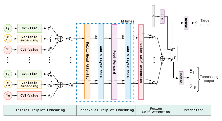
The architecture of STraTS is illustrated in Figure 3. Unlike most of the existing approaches which take a time-series matrix as input, STraTS defines its input as a set of observation triplets. Each observation triplet in the input is embedded using the Initial Triplet Embedding module. The initial triplet embeddings are then passed through a Contextual Triplet Embedding module which utilizes the Transfomer architecture to encode the context for each triplet. The Fusion Self-attention module then combines these contextual embeddings via self-attention mechanism to generate an embedding for the input time-series which is concatenated with demographics embedding and passed through a feed-forward network to make the final prediction. The notations used in the paper are summarized in Table 1.
# 3.2.1. Initial Triplet Embedding
Given an input time-series 𝐓={(ti,fi,vi)}i=1n, the initial embedding for the ith triplet 𝐞𝐢∈ℝd is computed by summing the following component embeddings: (i) Feature embedding 𝐞𝐢𝐟∈ℝd, (ii) Value embedding 𝐞𝐢𝐯∈ℝd, and (iii) Time embedding 𝐞𝐢𝐭∈ℝd. In other words, 𝐞𝐢=𝐞𝐢𝐟+𝐞𝐢𝐯+𝐞𝐢𝐭∈ℝd. Feature embeddings 𝐞𝐟(⋅) are obtained from a simple lookup table similar to word embeddings. Since feature values and times are continuous unlike feature names which are categorical objects, we cannot use a lookup table to embed these continuous values unless they are categorized. Some researchers (Vaswani et al., 2017; Yin et al., 2020) have used sinusoidal encodings to embed continuous values. We propose a novel continuous value embedding (CVE) technique using a one-to-many Feed-Forward Network (FFN) with learnable parameters i.e., 𝐞𝐢𝐯=FFNv(vi), and 𝐞𝐢𝐭=FFNt(ti).
Both FFNs have one input neuron and d output neurons and a single hidden layer with ⌊d⌋ neurons and tanh(⋅) activation. They are of the form FFN(x)=Utanh(Wx+b) where the dimensions of weights {W,b,U} can be inferred from the size of hidden and output layers of the FFN. Unlike sinusoidal encodings with fixed frequencies, this technique offers more flexibility by allowing end-to-end learning of continuous value and time embeddings without the need to categorize them.
Figure 3. The overall architecture of the proposed STraTS model. The Input Triplet Embedding module embeds each observation triplet, the Contextual Triplet Embedding module encodes contextual information for the triplets, the Fusion Self-Attention module computes time-series embedding which is concatenated with demographics embedding and passed through a dense layer to generate predictions for target and self-supervision (forecasting) tasks.

Fully described in text.
Figure 3. The overall architecture of the proposed STraTS model. The Input Triplet Embedding module embeds each observation triplet, the Contextual Triplet Embedding module encodes contextual information for the triplets, the Fusion Self-Attention module computes time-series embedding which is concatenated with demographics embedding and passed through a dense layer to generate predictions for target and self-supervision (forecasting) tasks.
# 3.2.2. Contextual Triplet Embedding
The initial triplet embeddings {𝐞1,…,𝐞n} are then passed through a Transformer architecture (Vaswani et al., 2017) with M blocks, each containing a Multi-Head Attention (MHA) layer with h attention heads and a FFN with one hidden layer. Each block takes n input embeddings 𝐄∈ℝn×d and outputs the corresponding n output embeddings 𝐂∈ℝn×d that capture the contextual information. MHA layers use multiple attention heads to attend to information contained in different embedding projections in parallel. The computations of the MHA layer are given by
# 3.2. Architecture of STraTS
The architecture of STraTS is illustrated in Figure 3. Unlike most of the existing approaches which take a time-series matrix as input, STraTS defines its input as a set of observation triplets. Each observation triplet in the input is embedded using the Initial Triplet Embedding module. The initial triplet embeddings are then passed through a Contextual Triplet Embedding module which utilizes the Transfomer architecture to encode the context for each triplet. The Fusion Self-attention module then combines these contextual embeddings via self-attention mechanism to generate an embedding for the input time-series which is concatenated with demographics embedding and passed through a feed-forward network to make the final prediction. The notations used in the paper are summarized in Table 1.
# 3.2.1. Initial Triplet Embedding
Given an input time-series 𝐓={(ti,fi,vi)}i=1n, the initial embedding for the ith triplet 𝐞𝐢∈ℝd is computed by summing the following component embeddings: (i) Feature embedding 𝐞𝐢𝐟∈ℝd, (ii) Value embedding 𝐞𝐢𝐯∈ℝd, and (iii) Time embedding 𝐞𝐢𝐭∈ℝd. In other words, 𝐞𝐢=𝐞𝐢𝐟+𝐞𝐢𝐯+𝐞𝐢𝐭∈ℝd. Feature embeddings 𝐞𝐟(⋅) are obtained from a simple lookup table similar to word embeddings. Since feature values and times are continuous unlike feature names which are categorical objects, we cannot use a lookup table to embed these continuous values unless they are categorized. Some researchers (Vaswani et al., 2017; Yin et al., 2020) have used sinusoidal encodings to embed continuous values. We propose a novel continuous value embedding (CVE) technique using a one-to-many Feed-Forward Network (FFN) with learnable parameters i.e., 𝐞𝐢𝐯=FFNv(vi), and 𝐞𝐢𝐭=FFNt(ti).
Both FFNs have one input neuron and d output neurons and a single hidden layer with ⌊d⌋ neurons and tanh(⋅) activation. They are of the form FFN(x)=Utanh(Wx+b) where the dimensions of weights {W,b,U} can be inferred from the size of hidden and output layers of the FFN. Unlike sinusoidal encodings with fixed frequencies, this technique offers more flexibility by allowing end-to-end learning of continuous value and time embeddings without the need to categorize them.
Figure 3. The overall architecture of the proposed STraTS model. The Input Triplet Embedding module embeds each observation triplet, the Contextual Triplet Embedding module encodes contextual information for the triplets, the Fusion Self-Attention module computes time-series embedding which is concatenated with demographics embedding and passed through a dense layer to generate predictions for target and self-supervision (forecasting) tasks.

Fully described in text.
Figure 3. The overall architecture of the proposed STraTS model. The Input Triplet Embedding module embeds each observation triplet, the Contextual Triplet Embedding module encodes contextual information for the triplets, the Fusion Self-Attention module computes time-series embedding which is concatenated with demographics embedding and passed through a dense layer to generate predictions for target and self-supervision (forecasting) tasks.
# 3.2.2. Contextual Triplet Embedding
The initial triplet embeddings {𝐞1,…,𝐞n} are then passed through a Transformer architecture (Vaswani et al., 2017) with M blocks, each containing a Multi-Head Attention (MHA) layer with h attention heads and a FFN with one hidden layer. Each block takes n input embeddings 𝐄∈ℝn×d and outputs the corresponding n output embeddings 𝐂∈ℝn×d that capture the contextual information. MHA layers use multiple attention heads to attend to information contained in different embedding projections in parallel. The computations of the MHA layer are given by
| (1) | 𝐇j=softmax((𝐄𝐖jq)(𝐄𝐖jk)Td/h)(𝐄𝐖jv)j=1,…,h | ||
| (2) | MHA(𝐄)=(𝐇1∘…∘𝐇h)𝐖c |
Each head projects the input embeddings into query, key, and value subspaces using matrices {𝐖jq,𝐖jk,𝐖jv}⊂ℝd×dh. The queries and keys are then used to compute the attention weights which are used to compute weighted averages of value (different from value in observation triplet) vectors. Finally, the outputs of all heads are concatenated and projected to original dimension with 𝐖c∈ℝhdh×d. The FFN layer takes the form
| (3) | 𝐅(𝐗) | =ReLU(𝐗𝐖1f+𝐛1f)𝐖2f+𝐛2f |
with weights 𝐖𝟏𝐟∈ℝd×2d,𝐛𝟏𝐟∈ℝ2d,𝐖𝟐𝐟∈ℝ2d×d,𝐛𝟐𝐟∈ℝd. Dropout, residual connections, and layer normalization are added for every MHA and FFN layer. Also, attention dropout randomly masks out some positions in the attention matrix before the softmax computation during training. The output of each block is fed as input to the succeeding one, and the output of the last block gives the contextual triplet embeddings {𝐜1,…,𝐜n}.
# 3.2.3. Fusion Self-attention
After computing contextual embeddings using a Transformer, we fuse them using a self-attention layer to compute time-series embedding 𝐞T∈ℝd. This layer first computes attention weights {α1,…,αn} by passing each contextual embedding through a FFN and computing a softmax over all the FFN outputs.
| (4) | ai | =𝐮aTtanh(𝐖a𝐜i+𝐛a) | ||
| (5) | αi | =exp(ai)∑j=1nexp(aj)∀i=1,…,n |
𝐖a∈ℝda×d,𝐛a∈ℝda,𝐮𝐚∈ℝda are the weights of this attention network which has da neurons in the hidden layer. The time-series embedding is then computed as
| (6) | 𝐞T=∑i=1nαi𝐜𝐢 |
# 3.2.4. Demographics Embedding
We realize that demographics can be encoded as triplets with a default value for time. However, we found that the prediction models performed better in our experiments when demographics are processed separately by passing 𝐝 through a FFN as shown below. The demographics embedding is thus obtained as
| (7) | 𝐞d=tanh(𝐖2dtanh(𝐖1d𝐝+𝐛1d)+𝐛2d)∈ℝd |
where the hidden layer has a dimension of 2d.
# 3.2.5. Prediction Head
The final prediction for target task is obtained by passing the concatenation of demographics and time-series embeddings through a dense layer with weights 𝐰oT∈ℝd, bo∈ℝ and sigmoid activation.
| (8) | y~=sigmoid(𝐰oT[𝐞d∘𝐞T]+bo) |
The model is trained on the target task using cross-entropy loss.